
at the Scripps Institution of Oceaongraphy
 |
Accelerated Climate Prediction Initiative (ACPI)
Pilot Program
at the Scripps Institution of Oceaongraphy |
Back to main page for pilot-ACPI at Scripps
SIO Contribution to pilot-ACPI quarterly progress report, 10-26-2000
1. Objectives
The objective of this phase of the project was to produce a restart file for the Parallel Coupled Model (PCM) that fulfilled two requirements:
The purpose of the second requirement, of drift small compared to the forced response, is so that the climate signal of interest can be discerned. Since the forcing consists of greenhouse gases that continually increase over the period of interest (1995-2100), it is likely that the response will have an important component that undergoes secular change as well. A climate drift from thermodynamically mismatched initial conditions would appear as a secular climate change, and so mask the signal of interest.
2. Approach
The approach we took to obtaining a model restart file with the required properties was to start with three-dimensional temperature and salinity fields from the ocean state estimation performed by D. Stammer (SIO/UCSD) as part of the NOPP funded ECCO Project (http://www.ecco.ucsd.edu). This will henceforth be referred to as the "assimilated data". The assimilated data cover the period 1992-1997, but the beginning of the run appeared to us to still have some model drift. Therefore, we averaged the years 1994-1997 to obtain three-dimensional oceanic fields of absolute temperature and salinity. Additionally, we intentionally tried to minimize the unwanted effects of either decadal climate variability or deep model drift on the results by only keeping data between 250 and 1500 meters depth.
Prior experience from many groups, ours included, suggests that it is futile to try to put absolute temperature fields from some external source directly into a coupled model. There is basically no chance that the implied atmospheric heat transport needed to maintain the absolute temperature field, and freshwater flux required to maintain the salinity field, will happen to match that actually produced by the atmospheric model. The result is invariably a strong climate drift to a different state, which would violate our objective #2 (described above).
Instead of using the absolute temperature and salinity fields of the assimilated data directly, we turned them into anomalies by subtracting off the three-dimensional Levitus fields of temperature and salinity. We then added these anomaly fields to the PCM's climatology to form the observation-based initial conditions. In this particular case the Levitus fields are the correct ones to take anomalies with respect to, because the assimilation run starts from Levitus' fields and then incorporates observed data on top of this using inverse techniques. Nevertheless, this step cannot be fully justified a priori. For one thing, the exact initial date of the Levitus initial conditions is not well defined since it incorporates data from many different years, but it is certain to reflect conditions later than the true pre-industrial state of 1870 or so. Mitigating this to some degree is the fact that there will be a appreciable thermal lag between the surface forcing and the mid-level response that we confine ourselves to (250 to 1500 m), and the majority of the observed warming between 1900 and 1995 occurred after 1970. Another possible problem is that a strongly inaccurate assimilation might result in final departures from the Levitus initial conditions that do not reflect surface forcing at all, but rather the inaccurate physics. For these reasons the reasonableness of the initial conditions we derived from the assimilated data must be checked.
2.1 Checking the Initial Conditions for Reasonableness
Checking the derived initial conditions is problematical in itself. Both the Levitus observations and the surface data used in the assimilation already go into the product, and so do not provide any independent information for checking their validity. In fact, since any observation-based data set could reasonably be expected to use as much data as is available, and therefore incorporate the Levitus data set, it is probably fair to say that there does not exist any truly independent observed data set to compare to.
We instead decided to check the reasonableness of the observation-based initial conditions by comparing them to historical and BAU runs of the PCM. Obviously, all this can tell us is whether or not the PCM's version of temperature changes due to anthropogenic gas forcing is consistent with the observation-based initial conditions. It is not possible to verify the initial conditions in an absolute sense. However, the PCM results are a completely independent data set, so agreement with the observation-based dataset would be meaningful. Also, since our objective is to construct initial conditions for PCM, significant disagreement between the oceanic global warming signal predicted by PCM and that seen the initial conditions data set would not bode well for starting PCM from the initial conditions, even if the initial conditions were assumed to be correct.
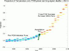
The first test we did of the PCM and observation-based initial conditions started by constructing the PCM's 3-dimensional (250 to 1500 m) oceanic global warming signal in year 2100, as a temperature anomaly from the time average of the PCM control run. Let this be denoted by P(2100). We then formed the projection of P(2100) on all prior years in the PCM run as follows:
Projection(y) = P(2100)*P(y) / (P(2100)*P(2100)),
where P(y) is PCM's temperature anomaly field at the prior year of interest, y. This dimensionless quantity will show "how much" of the global warming signal is already present at year y. The results are shown in Figure 1. The various colored bars denote different particular ensemble members for the historical and BAU runs of PCM. Ten years of model data goes into each colored bar. Basically, the run starts in year 1870 with none of the global warming signal present, has about 0.2 of the signal present by year 1995, and ends at 2100 with it all present.
 Figure
1: Projection of global warming signal
To compare this to the temperature anomaly fields from the assimilated data set, we calculated the same projection as above, but using A(y), the assimilated field at year y, instead of P(y). The results are shown as the green dots of Figure 1. With the exception of the initial years where the assimilation model is still spinning up, the projection values for the initial conditions fall on top of PCM's curve, indicating that the initial conditions contain about as much of the global warming signal in 1995 as the PCM model does.
This in itself is not a sufficient check. It is possible to have the right projection for the wrong reason, if, for example, A(y) were to contain a very strong but substantially incorrect pattern that happens to have a projection onto P(2100). To check for this possibility, we also did a straight pattern correlation between A(y) and P(2100), as shown in Figure 2 (note that the color scales are different in the two panels). We do not in this application care about small-scale differences, so the data has been spatially filtered to retain approximately 12 degrees of freedom.
The pattern correlation between the two is 0.56, which is significant at the 95% level with 12 dof. Additionally, a simple visual check confirms the results of the projection that the amplitude of A(y), the top panel, is about 0.2 times that of P(2100), the bottom panel. Thus we see that both the strength and the pattern of the observation-based initial condition data set matches that obtained from PCM. We therefore determined to proceed with using this initial condition data set directly in PCM.
3. Model Initialization Technique
Some care was taken to minimize possibility of shock when inserting this initial condition into PCM.
Firstly, both the temperature and salinity fields from the assimilation data set were used. This was to make sure that density changes, the dynamically important quantity, would be represented correctly.
Secondly, note that we have up to now restricted ourselves to the depth range 250-1500 m. This is to reduce the effects of decadal climate variability, which are more prominent in the upper, wind-driven layers of the ocean, and to isolate our results from any deep drift in the assimilation, where there is little observed data to constrain the results. But in order to avoid any "edge effects" from having vertical temperature anomalies jump instantaneously from zero to the imposed conditions as the 250 m boundary is passed, when constructing the restart data set for the model the fields were linearly ramped to zero, starting at 250 m and ending beneath the first layer (~25 m).
Thirdly, inserting the temperature and salinity (and therefore, density) anomaly fields into the model will result in the geostrophic velocities being out of balance with the density field when the model first starts, resulting in a shock. Additionally, we did not modify the ice field, which must also adjust to the imposed initial conditions. For these reasons we started the model with the constructed T,S fields in year 1995, but then continued to strongly (30-day time scale) relax the model to these conditions (taking the seasonal variability of the model into account) until the end of year 1999. Only the ocean T and S fields were relaxed; this allowed the ocean velocity field, and the entire ice and atmospheric components of the coupled model, to adjust as needed to be self-consistent with these initial conditions. We then instantaneously removed the relaxation to our calculated T, S fields, and let the model integrate forward as usual.
4. Model Variability and Drift after Initialization
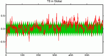
The second objective was to make sure that the model variability was within reasonable limits, and any model drift was small compared to the forced signal of interest. To do this, we let the model integrate forward for 50 years with constant surface forcing corresponding to year 1995, and compared the results to the PCM runs forced with BAU scenarios. The full set of results can be found in http://meteora.ucsd.edu/~pierce/plots/acpi/assim/. Figure 3 shows one of this set, a simple but useful diagnostic, the global mean temperature anomaly (degrees C).
 Figure
3: Global surface temperature
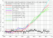
The green region is +/- 1.5 times the standard deviation of TS by month, calculated from the ensemble of five historical PCM runs over the period 1990-1999 (50 years total data). This gives a measure of the natural variability to be expected. It can be seen that there is substantial variability, as expected from the BAU scenarios, and a weak drift of about 0.2 C during the 50 years. Figure 4, courtesy of Aiguo Dai of NCAR, show the results for an ensemble of PCM model runs with anthropogenic forcing.
 Figure
4: PCM control and BAU runs
The substantial interannual and decadal variability is again evident in the control run (black line). At year 2000, the surface temperature anomaly in the BAU runs (red line) is about 0.6 C; in year 2050, it is about 1.6 C. Therefore, over 50 years the forced signal is about 1.0 C, or about 5 times the drift seen in the test run. The drift seen using the observation-based initial conditions is sufficiently small to proceed with the production runs.
A final thing to note about this residual model drift is that there is no reason to think that the model's climate state in year 1995 is in equilibrium. Since the rate of change of greenhouse gases is appreciable at that time, and there is a decadal-timescale time lag between temperatures in the middle ocean and the surface forcing, there is every reason to think that the ocean will still adjust by warming for some decades even if surface conditions are held fixed at 1995 values. The residual drift in the test run may be no more than this. If we have the computer resources, we intend to check this by simply integrating forward PCM from a year 1995 restart file with fixed surface conditions.
5. Summary: Coupled Model Initialization